Contents
- Sorting Algorithms
- Timing the code
- The Bubble Sort Algorithm
- The Insertion Sort Algorithm
- The Merge Sort Algorithm
- The Quicksort Algorithm
- Selecting the pivot Element
- Measuring Quicksort’s Big O Complexity
- Analyzing the Strengths and Weaknesses of Quicksort
- The Timsort Algorithm
- Modified Insertion Sort
- Time sort
- Measuring Timsort’s Big O Complexity
- Analyzing the Strengths and Weaknesses of Timsort
- Comparision
- Sorting can be used to solve multiple problems
Searching: Searching for an item on a list works much faster if the list is sorted.
Selection: Selecting items from a list based on their relationship to the rest of the items is easier with sorted data. For example, finding the kth-largest or smallest value, or finding the median value of the list, is much easier when the values are in ascending or descending order.
Duplicates: Finding duplicate values on a list can be done very quickly when the list is sorted.
Distribution: Analyzing the frequency distribution of items on a list is very fast if the list is sorted.
Timing the code
from random import randint

from timeit import repeat


def run_sorting_algorithm(algorithm, array):

    # Set up the context and prepare the call to the specified
    # algorithm using the supplied array. Only import the
    # algorithm function if it's not the built-in `sorted()`.
    setup_code = f"from __main__ import {algorithm}" if algorithm != "sorted" else ""

    stmt = f"{algorithm}({array})"


    # Execute the code ten different times and return the time
    # in seconds that each execution took
    times = repeat(setup=setup_code, stmt=stmt, repeat=3, number=10)


    # Finally, display the name of the algorithm and the
    # minimum time it took to run

    print(f"Algorithm: {algorithm}. Minimum execution time: {min(times)}")
Measuring Efficiency With Big O Notation
The time in seconds required to run different algorithms can be influenced by several unrelated factors, including processor speed or available memory. Big O, on the other hand, provides a platform to express runtime complexity in hardware-agnostic terms.
With Big O, you express complexity in terms of how quickly your algorithm’s runtime grows relative to the size of the input, especially as the input grows arbitrarily large.
The Bubble Sort Algorithm
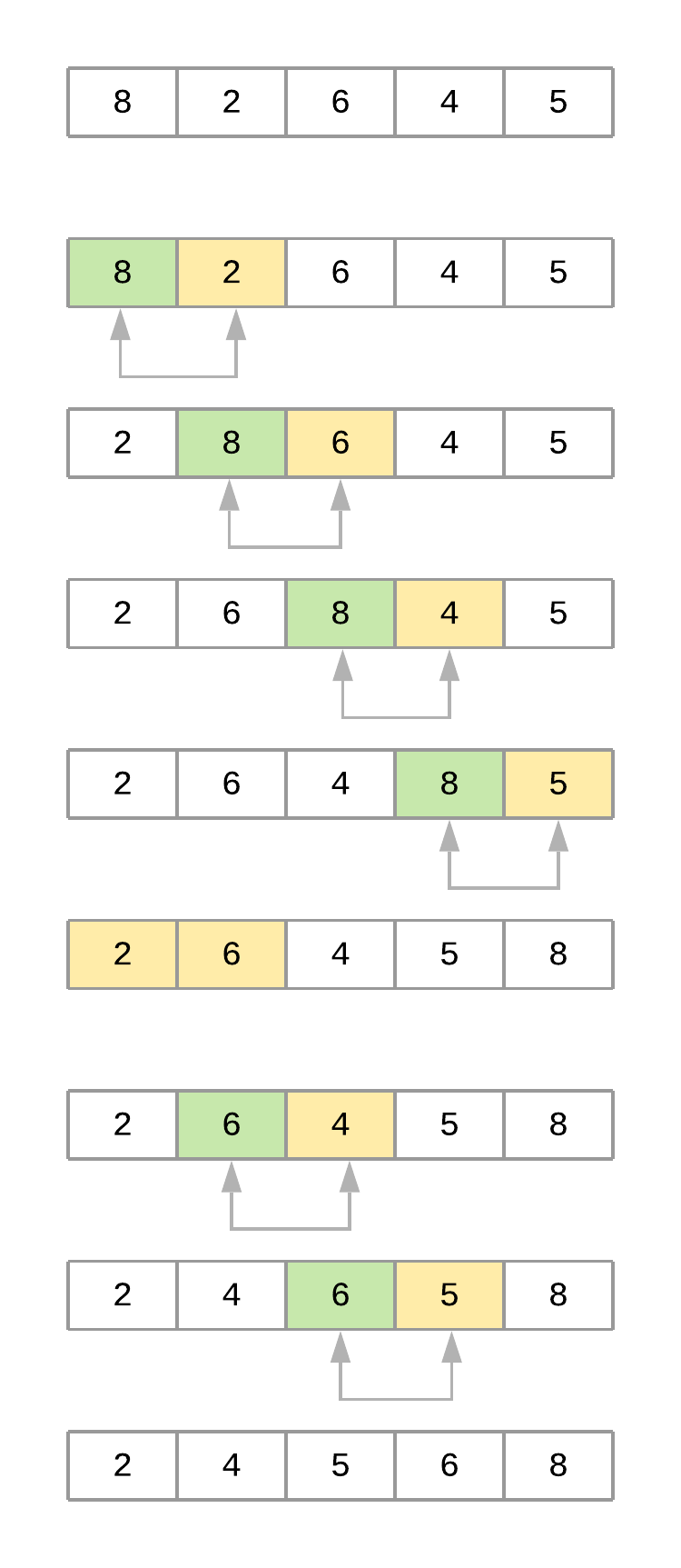
Bubble Sort is one of the most straightforward sorting algorithms. Its name comes from the way the algorithm works: With every new pass, the largest element in the list “bubbles up” toward its correct position.
Bubble sort consists of making multiple passes through a list, comparing elements one by one, and swapping adjacent items that are out of order.
def bubble_sort(array):

    n = len(array)


    for i in range(n):

        # Create a flag that will allow the function to
        # terminate early if there's nothing left to sort
        already_sorted = True


        # Start looking at each item of the list one by one,
        # comparing it with its adjacent value. With each
        # iteration, the portion of the array that you look at
        # shrinks because the remaining items have already been
        # sorted.
        for j in range(n - i - 1):


            if array[j] > array[j + 1]:

                # If the item you're looking at is greater than its
                # adjacent value, then swap them
                array[j], array[j + 1] = array[j + 1], array[j]


                # Since you had to swap two elements,
                # set the `already_sorted` flag to `False` so the
                # algorithm doesn't finish prematurely
                already_sorted = False

            # print(array)


        # If there were no swaps during the last iteration,
        # the array is already sorted, and you can terminate
        if already_sorted:

            break


    return array
bubble_sort([10,9,8,7,6,5,4,3,2,1])
- Since this implementation sorts the array in ascending order, each step “bubbles” the largest element to the end of the array. This means that each iteration takes fewer steps than the previous iteration because a continuously larger portion of the array is sorted.
- Notice how j initially goes from the first element in the list to the element immediately before the last. During the second iteration, j runs until two items from the last, then three items from the last, and so on. At the end of each iteration, the end portion of the list will be sorted.
Note: The already_sorted flag is an optimization to the algorithm, and it’s not required in a fully functional bubble sort implementation. However, it allows the function to save unnecessary steps if the list ends up wholly sorted before the loops have finished.
Measuring Bubble Sort’s Big O Runtime Complexity
Your implementation of bubble sort consists of two nested for loops in which the algorithm performs n - 1 comparisons, then n - 2 comparisons, and so on until the final comparison is done. This comes at a total of (n - 1) + (n - 2) + (n - 3) + … + 2 + 1 = n(n-1)/2 comparisons, which can also be written as ½$n^2$ - ½n.
You learned earlier that Big O focuses on how the runtime grows in comparison to the size of the input. That means that, in order to turn the above equation into the Big O complexity of the algorithm, you need to remove the constants because they don’t change with the input size.
Doing so simplifies the notation to n2 - n. Since $n^2$ grows much faster than n, this last term can be dropped as well, leaving bubble sort with an average- and worst-case complexity of $\boldsymbol{O(n^2)}$.
In cases where the algorithm receives an array that’s already sorted—and assuming the implementation includes the already_sorted flag optimization explained before—the runtime complexity will come down to a much better O(n) because the algorithm will not need to visit any element more than once.
O(n), then, is the best-case runtime complexity of bubble sort. But keep in mind that best cases are an exception, and you should focus on the average case when comparing different algorithms.
The Insertion Sort Algorithm
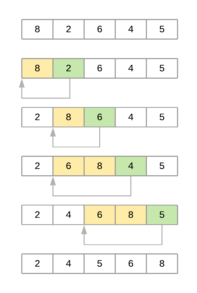
- Like bubble sort, the insertion sort algorithm is straightforward to implement and understand. But unlike bubble sort, it builds the sorted list one element at a time by comparing each item with the rest of the list and inserting it into its correct position. This “insertion” procedure gives the algorithm its name.
- An excellent analogy to explain insertion sort is the way you would sort a deck of cards. Imagine that you’re holding a group of cards in your hands, and you want to arrange them in order. You’d start by comparing a single card step by step with the rest of the cards until you find its correct position. At that point, you’d insert the card in the correct location and start over with a new card, repeating until all the cards in your hand were sorted.
def insertion_sort(array):

    # Loop from the second element of the array until
    # the last element

    for i in range(1, len(array)):

        # This is the element we want to position in its
        # correct place
        key_item = array[i]


        # Initialize the variable that will be used to
        # find the correct position of the element referenced
        # by `key_item`
        j = i - 1


        # Run through the list of items (the left
        # portion of the array) and find the correct position
        # of the element referenced by `key_item`. Do this only
        # if `key_item` is smaller than its adjacent values.
        while j >= 0 and array[j] > key_item:

            # Shift the value one position to the left
            # and reposition j to point to the next element
            # (from right to left)
            array[j + 1] = array[j]
            j -= 1

            # print(array, i , j)


        # When you finish shifting the elements, you can position
        # `key_item` in its correct location
        array[j + 1] = key_item

    return array
insertion_sort([10,9,8,7,6,5,4,3,2,1])
Note: Unlike bubble sort, this implementation of insertion sort constructs the sorted list by pushing smaller items to the left.
Measuring Insertion Sort’s Big O Runtime Complexity
Similar to your bubble sort implementation, the insertion sort algorithm has a couple of nested loops that go over the list. The inner loop is pretty efficient because it only goes through the list until it finds the correct position of an element. That said, the algorithm still has an $\boldsymbol{O(n^2)}$ runtime complexity on the average case.
The worst case happens when the supplied array is sorted in reverse order. In this case, the inner loop has to execute every comparison to put every element in its correct position. This still gives you an $\boldsymbol{O(n^2)}$ runtime complexity.
The best case happens when the supplied array is already sorted. Here, the inner loop is never executed, resulting in an O(n) runtime complexity, just like the best case of bubble sort.
Although bubble sort and insertion sort have the same Big O runtime complexity, in practice, insertion sort is considerably more efficient than bubble sort. If you look at the implementation of both algorithms, then you can see how insertion sort has to make fewer comparisons to sort the list.
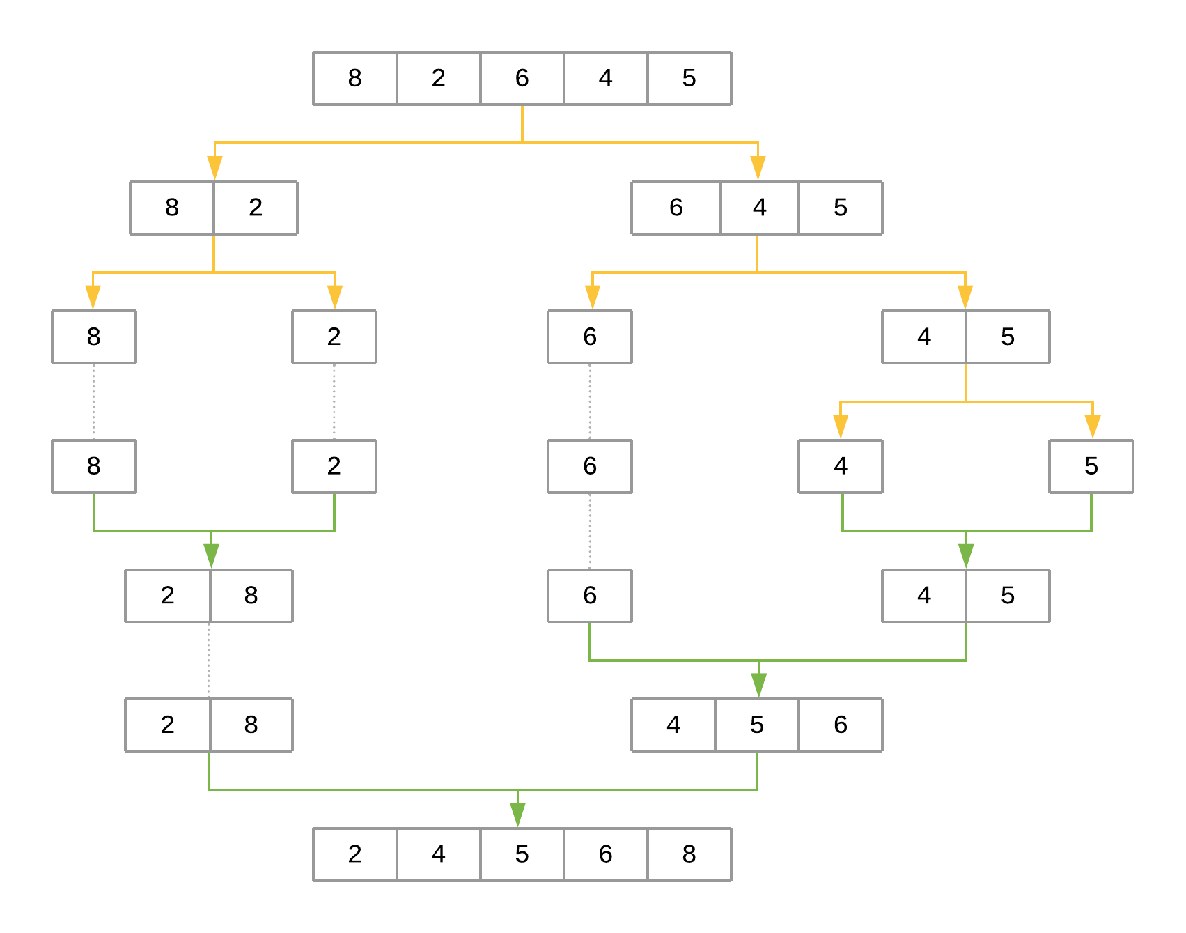
The Merge Sort Algorithm
In the case of merge sort, the divide-and-conquer approach divides the set of input values into two equal-sized parts, sorts each half recursively, and finally merges these two sorted parts into a single sorted list.
The implementation of the merge sort algorithm needs two different pieces:
- A function that recursively splits the input in half
- A function that merges both halves, producing a sorted array
def merge(left, right):

    # If the first array is empty, then nothing needs
    # to be merged, and you can return the second array as the result
    if len(left) == 0:

        return right


    # If the second array is empty, then nothing needs
    # to be merged, and you can return the first array as the result
    if len(right) == 0:

        return left


    result = []

    index_left = index_right = 0

    # Now go through both arrays until all the elements
    # make it into the resultant array
    while len(result) < len(left) + len(right):

        # The elements need to be sorted to add them to the
        # resultant array, so you need to decide whether to get
        # the next element from the first or the second array
        if left[index_left] <= right[index_right]:

            result.append(left[index_left])

            index_left += 1

        else:

            result.append(right[index_right])

            index_right += 1


        # If you reach the end of either array, then you can
        # add the remaining elements from the other array to
        # the result and break the loop
        if index_right == len(right):

            result += left[index_left:]

            break


        if index_left == len(left):

            result += right[index_right:]

            break


    return result
- With the above function in place, the only missing piece is a function that recursively splits the input array in half and uses merge() to produce the final result:
def merge_sort(array):

    # If the input array contains fewer than two elements,
    # then return it as the result of the function
    if len(array) < 2:

        return array


    midpoint = len(array) // 2

    # Sort the array by recursively splitting the input
    # into two equal halves, sorting each half and merging them
    # together into the final result

    return merge(

        left=merge_sort(array[:midpoint]),

        right=merge_sort(array[midpoint:]))
merge_sort([8, 2, 6, 4, 5])
Measuring Merge Sort’s Big O Complexity
To analyze the complexity of merge sort, you can look at its two steps separately:
merge() has a linear runtime. It receives two arrays whose combined length is at most n (the length of the original input array), and it combines both arrays by looking at each element at most once. This leads to a runtime complexity of O(n).
The second step splits the input array recursively and calls merge() for each half. Since the array is halved until a single element remains, the total number of halving operations performed by this function is $\boldsymbol{log_2n}$. Since merge() is called for each half, we get a total runtime of $\boldsymbol{O(n log_2n)}$.
Interestingly, $\boldsymbol{O(n log_2n)}$ is the best possible worst-case runtime that can be achieved by a sorting algorithm.
Drawbacks of merge sort:
for small lists, the time cost of the recursion allows algorithms such as bubble sort and insertion sort to be faster.
Another drawback of merge sort is that it creates copies of the array when calling itself recursively. It also creates a new list inside merge() to sort and return both input halves. This makes merge sort use much more memory than bubble sort and insertion sort, which are both able to sort the list in place.
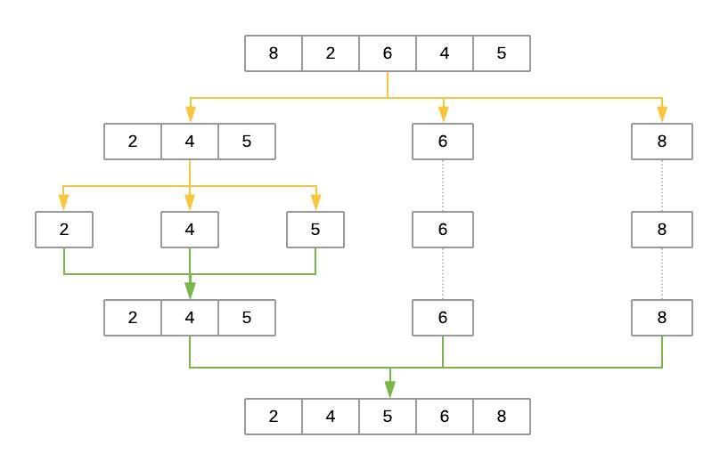
The Quicksort Algorithm
Just like merge sort, the Quicksort algorithm applies the divide-and-conquer principle to divide the input array into two lists, the first with small items and the second with large items. The algorithm then sorts both lists recursively until the resultant list is completely sorted.
Dividing the input list is referred to as partitioning the list. Quicksort first selects a pivot element and partitions the list around the pivot, putting every smaller element into a low array and every larger element into a high array.
Putting every element from the low list to the left of the pivot and every element from the high list to the right positions the pivot precisely where it needs to be in the final sorted list. This means that the function can now recursively apply the same procedure to low and then high until the entire list is sorted.
from random import randint


def quicksort(array):

    # If the input array contains fewer than two elements,
    # then return it as the result of the function
    if len(array) < 2:

        return array


    low, same, high = [], [], []


    # Select your `pivot` element randomly
    pivot = array[randint(0, len(array) - 1)]


    for item in array:

        # Elements that are smaller than the `pivot` go to
        # the `low` list. Elements that are larger than
        # `pivot` go to the `high` list. Elements that are
        # equal to `pivot` go to the `same` list.
        if item < pivot:

            low.append(item)

        elif item == pivot:

            same.append(item)

        elif item > pivot:

            high.append(item)


    # The final result combines the sorted `low` list
    # with the `same` list and the sorted `high` list
    return quicksort(low) + same + quicksort(high)
quicksort([8, 2, 6, 4, 5])
Note: Above pivot element is selected randomly, it's a coincidence that it is every time the middle one
Selecting the pivot Element
Why does the implementation above select the pivot element randomly? Wouldn’t it be the same to consistently select the first or last element of the input list?
Because of how the Quicksort algorithm works, the number of recursion levels depends on where pivot ends up in each partition. In the best-case scenario, the algorithm consistently picks the median element as the pivot. That would make each generated subproblem exactly half the size of the previous problem, leading to at most $\boldsymbol{log_2n}$ levels.
On the other hand, if the algorithm consistently picks either the smallest or largest element of the array as the pivot, then the generated partitions will be as unequal as possible, leading to n-1 recursion levels. That would be the worst-case scenario for Quicksort.
As you can see, Quicksort’s efficiency often depends on the pivot selection. If the input array is unsorted, then using the first or last element as the pivot will work the same as a random element. But if the input array is sorted or almost sorted, using the first or last element as the pivot could lead to a worst-case scenario. Selecting the pivot at random makes it more likely Quicksort will select a value closer to the median and finish faster.
Another option for selecting the pivot is to find the median value of the array and force the algorithm to use it as the pivot. This can be done in O(n) time. Although the process is little bit more involved, using the median value as the pivot for Quicksort guarantees you will have the best-case Big O scenario.
Measuring Quicksort’s Big O Complexity
With Quicksort, the input list is partitioned in linear time, O(n), and this process repeats recursively an average of $\boldsymbol{log_2n}$ times. This leads to a final complexity of $\boldsymbol{O(n log_2n)}$.
That said, remember the discussion about how the selection of the pivot affects the runtime of the algorithm. The O(n) best-case scenario happens when the selected pivot is close to the median of the array, and an O($n^2$) scenario happens when the pivot is the smallest or largest value of the array.
Theoretically, if the algorithm focuses first on finding the median value and then uses it as the pivot element, then the worst-case complexity will come down to $\boldsymbol{O(n log_2n)}$. The median of an array can be found in linear time, and using it as the pivot guarantees the Quicksort portion of the code will perform in $\boldsymbol{O(n log_2n)}$.
By using the median value as the pivot, you end up with a final runtime of O(n) + $\boldsymbol{O(n log_2n)}$. You can simplify this down to $\boldsymbol{O(n log_2n)}$ because the logarithmic portion grows much faster than the linear portion.
Analyzing the Strengths and Weaknesses of Quicksort
True to its name, Quicksort is very fast. Although its worst-case scenario is theoretically O(n2), in practice, a good implementation of Quicksort beats most other sorting implementations. Also, just like merge sort, Quicksort is straightforward to parallelize.
One of Quicksort’s main disadvantages is the lack of a guarantee that it will achieve the average runtime complexity. Although worst-case scenarios are rare, certain applications can’t afford to risk poor performance, so they opt for algorithms that stay within O(n log2n) regardless of the input.
Just like merge sort, Quicksort also trades off memory space for speed. This may become a limitation for sorting larger lists.
The Timsort Algorithm
The Timsort algorithm is considered a hybrid sorting algorithm because it employs a best-of-both-worlds combination of insertion sort and merge sort. Timsort is near and dear to the Python community because it was created by Tim Peters in 2002 to be used as the standard sorting algorithm of the Python language.
The main characteristic of Timsort is that it takes advantage of already-sorted elements that exist in most real-world datasets. These are called natural runs. The algorithm then iterates over the list, collecting the elements into runs and merging them into a single sorted list.
Modified Insertion Sort
# The first step in implementing Timsort is modifying the implementation of insertion_sort() from before

def insertion_sort(array, left=0, right=None):

    if right is None:

        right = len(array) - 1


    # Loop from the element indicated by
    # `left` until the element indicated by `right`
    for i in range(left + 1, right + 1):

        # This is the element we want to position in its
        # correct place
        key_item = array[i]


        # Initialize the variable that will be used to
        # find the correct position of the element referenced
        # by `key_item`
        j = i - 1


        # Run through the list of items (the left
        # portion of the array) and find the correct position
        # of the element referenced by `key_item`. Do this only
        # if the `key_item` is smaller than its adjacent values.
        while j >= left and array[j] > key_item:

            # Shift the value one position to the left
            # and reposition `j` to point to the next element
            # (from right to left)
            array[j + 1] = array[j]

            j -= 1


        # When you finish shifting the elements, position
        # the `key_item` in its correct location
        array[j + 1] = key_item


    return array
insertion_sort([8, 2, 6, 4, 5])
Note: This modified implementation adds a couple of parameters, left and right, that indicate which portion of the array should be sorted. This allows the Timsort algorithm to sort a portion of the array in place.
Time sort
def timsort(array):

    min_run = 32

    n = len(array)


    # Start by slicing and sorting small portions of the
    # input array. The size of these slices is defined by
    # your `min_run` size.
    for i in range(0, n, min_run):

        insertion_sort(array, i, min((i + min_run - 1), n - 1))


    # Now you can start merging the sorted slices.
    # Start from `min_run`, doubling the size on
    # each iteration until you surpass the length of
    # the array.
    size = min_run

    while size < n:

        # Determine the arrays that will
        # be merged together
        for start in range(0, n, size * 2):

            # Compute the `midpoint` (where the first array ends
            # and the second starts) and the `endpoint` (where
            # the second array ends)
            midpoint = start + size - 1

            end = min((start + size * 2 - 1), (n-1))


            # Merge the two subarrays.
            # The `left` array should go from `start` to
            # `midpoint + 1`, while the `right` array should
            # go from `midpoint + 1` to `end + 1`.
            merged_array = merge(

                left=array[start:midpoint + 1],

                right=array[midpoint + 1:end + 1])


            # Finally, put the merged array back into
            # your array
            array[start:start + len(merged_array)] = merged_array


        # Each iteration should double the size of your arrays
        size *= 2


    return array
Measuring Timsort’s Big O Complexity
On average, the complexity of Timsort is $\boldsymbol{O(n log_2n)}$, just like merge sort and Quicksort. The logarithmic part comes from doubling the size of the run to perform each linear merge operation.
However, Timsort performs exceptionally well on already-sorted or close-to-sorted lists, leading to a best-case scenario of O(n). In this case, Timsort clearly beats merge sort and matches the best-case scenario for Quicksort. But the worst case for Timsort is also $\boldsymbol{O(n log_2n)}$, which surpasses Quicksort’s O($n^2$).
Analyzing the Strengths and Weaknesses of Timsort
The main disadvantage of Timsort is its complexity. Despite implementing a very simplified version of the original algorithm, it still requires much more code because it relies on both insertion_sort() and merge().
One of Timsort’s advantages is its ability to predictably perform in O(n log2n) regardless of the structure of the input array. Contrast that with Quicksort, which can degrade down to O(n2). Timsort is also very fast for small arrays because the algorithm turns into a single insertion sort.
For real-world usage, in which it’s common to sort arrays that already have some preexisting order, Timsort is a great option. Its adaptability makes it an excellent choice for sorting arrays of any length.
Comparision
ARRAY_LENGTH = 10000
- For not sorted array
array = [randint(0, 1000) for i in range(ARRAY_LENGTH)]

# Call each of the functions
run_sorting_algorithm(algorithm="bubble_sort", array=array)

run_sorting_algorithm(algorithm="insertion_sort", array=array)

run_sorting_algorithm(algorithm="merge_sort", array=array)

run_sorting_algorithm(algorithm="quicksort", array=array)

run_sorting_algorithm(algorithm="timsort", array=array)
- For already sorted array
array = [i for i in range(ARRAY_LENGTH)]

# Call each of the functions
run_sorting_algorithm(algorithm="bubble_sort", array=array)

run_sorting_algorithm(algorithm="insertion_sort", array=array)

run_sorting_algorithm(algorithm="merge_sort", array=array)

run_sorting_algorithm(algorithm="quicksort", array=array)

run_sorting_algorithm(algorithm="timsort", array=array)